Weibull model functions

'weibull' and 'weibull2' provide a very general way of specifying Weibull dose response functions, under various constraints on the parameters.

weibull1(fixed = c(NA, NA, NA, NA),
           names = c("b", "c", "d", "e"),
           method = c("1", "2", "3", "4"),
           ssfct = NULL,
           fctName, fctText)

  weibull2(fixed = c(NA, NA, NA, NA),
           names = c("b", "c", "d", "e"),
           method = c("1", "2", "3", "4"),
           ssfct = NULL,
           fctName, fctText)

  weibull2x(fixed = rep(NA, 5),
           names = c("b", "c", "d", "e", "t0"),
           method = c("1", "2", "3", "4"),
           ssfct = NULL,
           fctName, fctText)

Arguments

fixed	numeric vector. Specifies which parameters are fixed and at what value they are fixed. NAs for parameter that are not fixed.
names	a vector of character strings giving the names of the parameters (should not contain ":"). The default is reasonable (see under 'Usage'). The order of the parameters is: b, c, d, e (see under 'Details').
method	character string indicating the self starter function to use.
ssfct	a self starter function to be used.
fctName	optional character string used internally by convenience functions.
fctText	optional character string used internally by convenience functions.

Details

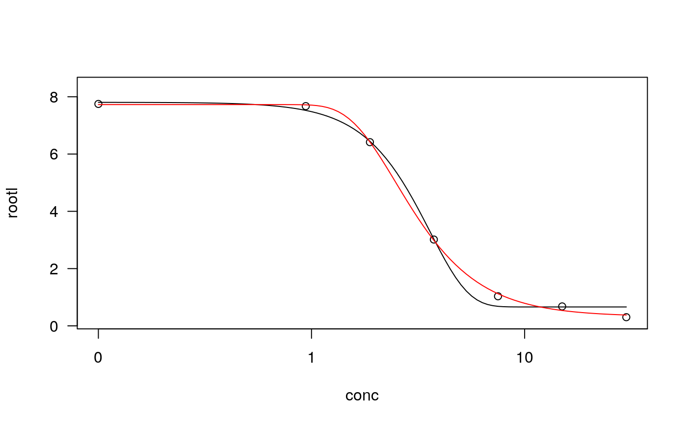
As pointed out in Seber and Wild (1989), there exist two different parameterisations of the Weibull model. They do not yield the same fitted curve for a given dataset (see under Examples).

The four-parameter Weibull type 1 model ('weibull1') is $$ f(x) = c + (d-c) \exp(-\exp(b(\log(x)-\log(e)))).$$

Thw four-parameter Weibull type 2 model ('weibull2') is $$ f(x) = c + (d-c) (1 - \exp(-\exp(b(\log(x)-\log(e))))).$$

Both four-parameter model functions are asymmetric with inflection point at the dose equal \(e\).

Value

The value returned is a list containing the non-linear function, the self starter function and the parameter names.

References

Seber, G. A. F. and Wild, C. J (1989) Nonlinear Regression, New York: Wiley \& Sons (pp. 338--339).

Note

The functions are for use with the function drm.

See also

For convenience several special cases of the function 'weibull1' are available: W1.2, W1.3 and W1.4.

Special cases of 'weibull2' are: W2.2, W2.3 and W2.4.

These convenience functions should be used rather than the underlying functions weibull1 and weibull2.

Examples

## Fitting two different Weibull models
ryegrass.m1 <- drm(ryegrass, fct = W1.4())
plot(ryegrass.m1, conLevel=0.5)
#> Warning: "conLevel" is not a graphical parameter
#> Warning: "conLevel" is not a graphical parameter
#> Warning: "conLevel" is not a graphical parameter
#> Warning: "conLevel" is not a graphical parameter
#> Warning: "conLevel" is not a graphical parameter

ryegrass.m2 <- drm(ryegrass, fct = W2.4())
plot(ryegrass.m2, conLevel=0.5, add = TRUE, type = "none", col = 2)
#> Warning: "conLevel" is not a graphical parameter
# you could also look at the ED values to see the difference

## A four-parameter Weibull model with b fixed at 1
ryegrass.m3 <- drm(ryegrass, fct = W1.4(fixed = c(1, NA, NA, NA)))
summary(ryegrass.m3)
#> 
#> Model fitted: Weibull (type 1) (3 parms)
#> 
#> Parameter estimates:
#> 
#>               Estimate Std. Error t-value   p-value    
#> c:(Intercept)  0.12945    0.36866  0.3511     0.729    
#> d:(Intercept)  8.23936    0.30335 27.1613 < 2.2e-16 ***
#> e:(Intercept)  4.53797    0.63886  7.1032 5.243e-07 ***
#> ---
#> Signif. codes:  0 ‘***’ 0.001 ‘**’ 0.01 ‘*’ 0.05 ‘.’ 0.1 ‘ ’ 1
#> 
#> Residual standard error:
#> 
#>  0.8384585 (21 degrees of freedom)

## A four-parameter Weibull model with the constraint b>3
ryegrass.m4 <- drm(ryegrass, fct = W1.4(), lowerl = c(3, -Inf, -Inf, -Inf),
control = drmc(constr=TRUE))
summary(ryegrass.m4)
#> 
#> Model fitted: Weibull (type 1) (4 parms)
#> 
#> Parameter estimates:
#> 
#>               Estimate Std. Error t-value   p-value    
#> b:(Intercept)  3.00000    0.82015  3.6579  0.001563 ** 
#> c:(Intercept)  0.68190    0.18943  3.5999  0.001789 ** 
#> d:(Intercept)  7.68189    0.23088 33.2719 < 2.2e-16 ***
#> e:(Intercept)  3.58441    0.16992 21.0951 3.946e-15 ***
#> ---
#> Signif. codes:  0 ‘***’ 0.001 ‘**’ 0.01 ‘*’ 0.05 ‘.’ 0.1 ‘ ’ 1
#> 
#> Residual standard error:
#> 
#>  0.5657677 (20 degrees of freedom)